Perinatal mortality - monthly data

Model

A model for the trend of monthly data has to allow for seasonal variations of perinatal mortality rates. Two periodic terms with periods of 12 and 6 months are therefore added to the long-term trend, and four additional parameters are needed, two for the amplitudes (β₄, β₆) and two for the phase shifts (β₅, β₇):

E(Y(t)) = 1/(1+1/exp(β₁ +β₂·t +β₃·t² +β₄·cos(2pi·(t-β₅)) +β₆·cos(2pi·(2t-β₇))))

The time variable t points to the centre of a month, where a "month" is defined as one twelfth of a year. To avoid large numbers, the time axis starts in 1980. May 1986, e.g., corresponds to t=6.375.

The caesium concentration in cow milk is used as a proxy for the total internal radiation exposure from caesium, essentially because data of caesium contamination in cow milk were available. The caesium concentrations in cow milk were measured at the Munich based GSF-Institute nearly every day, from the beginning of May 1986 until the end of 1988. In the first year following Chernobyl, the internal exposure of the German population, mainly from caesium in cow milk, exceeded the external caesium exposure. Milk produced in higher contaminated southern Bavaria was distributed and consumed throughout West Germany. In Berlin, where the caesium soil contamination was nearly 10-times smaller than in Munich, the average caesium content in individuals was only a factor of two lower than in Munich.

The calculation of the caesium concentration in pregnant women is based on the assumption of a constant daily milk consumption and a somewhat reduced biological half-life of caesium of 70 days during pregnancy. The caesium burden increases with caesium uptake and decreases with caesium excretion. Figure 1 shows the measured caesium concentration in milk (dots) and the calculated caesium burden in pregnant women (solid line).

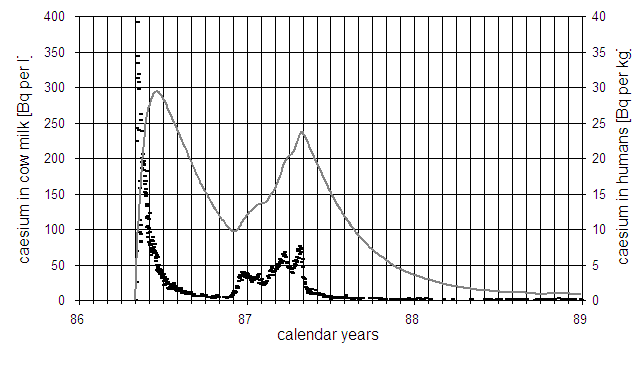
Fig.1: Caesium concentration in cow milk (short dashes) and in pregnant women (solid line), calculated with a constant daily consumption of cow milk and a biological half life of 70 days.

The regression model with the caesium term has the following form:

E(Y(t)) = 1/(1+1/exp(β₁ +β₂·t +β₃·t² +β₄·cos(2pi·(t-β₅)) +β₆·cos(2pi·(2t-β₇)) +β₈·(cs(t-β₁₀))^β₉))

Parameter β₈ is a constant, β₁₀ is the time-lag between caesium concentration cs(t) and perinatal mortality, and β₉ is the power of dose which allows for a curvilinear dose-response relationship.

To test the significance of the caesium term, the weighted sum of squares resulting from a regression with the full model is compared with the sum of squares obtained from a regression without the caesium term. An F-test is applied to test the significance of the caesium term. The test statistic is

F = ((χ²₀-χ²₁)/(df₀-df₁))/(χ²₁/df₁)

where χ²₀ and χ²₁ denote the weighted sum of squares under the null hypothesis and under the full model, respectively; df₀ and df₁ are the corresponding degrees of freedom. Here df₀-df₁ equals the number of parameters to be tested.

Perinatal mortality in Germany

A regression without the caesium term yields a weighted sum of squares of 221.6 (df=161). Regressions with the full model are then performed with different time-lags β₁₀. The best fit with a sum of squares of 204.5 (df=158) is obtained for a time-lag of 7 months. The corresponding F-test is significant (p=0.0053).

Figure 2 shows German monthly perinatal mortality rates and the long-term trend. Figure 3 displays the deviations of the observed rates from the calculated undisturbed trend (standardised residuals) and the three-month moving average. There are significant peaks of perinatal mortality in the beginning and at the end of 1987.

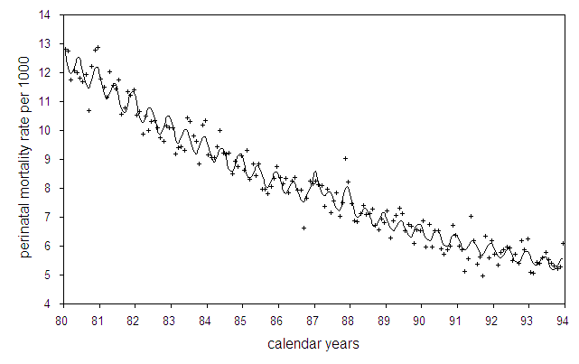
Fig.2: Monthly perinatal mortality rates in Germany and regression line with seasonal fluctuations

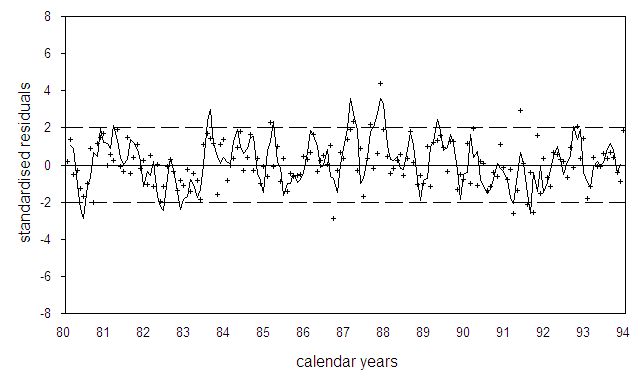
Fig.3: Deviation of monthly perinatal mortality rates in Germany from the undisturbed long-term trend of the data in units of standard deviations (standardized residuals). The solid line is the three-month moving average, the broken lines show the range of two standard deviations.

In Figure 4, the profile sum of squares is plotted as a function of the time-lag. The broken line gives an estimate of the 95% confidence interval from 5.5 to 8.5 months based on the F-test.

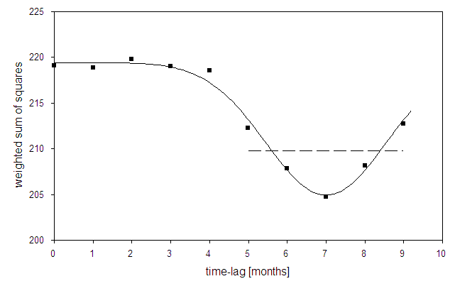
Fig.4: Sum of squares as a function of the time-lag between caesium concentration in pregnant women and perinatal mortality in Germany (profile likelihood). The broken line indicates the 95% confidence interval for the time-lag ranging from 5.5 to 8.5 months.

Perinatal mortality in Zhitomir oblast, Ukraine

The Ukrainian region (oblast) Zhitomir is the most contaminated region of Ukraine. But due to the small number of inhabitants (1.4 mio) it is not easy to detect deviations from the expected trend.

Figure 5 shows the deviations of monthly perinatal mortality rates in Zhitomir from the trend of the years 1985-1991 without 1987. There are peaks of perinatal mortality in January and in April 1987 which coincide with peaks of infant mortality peaks in Poland.

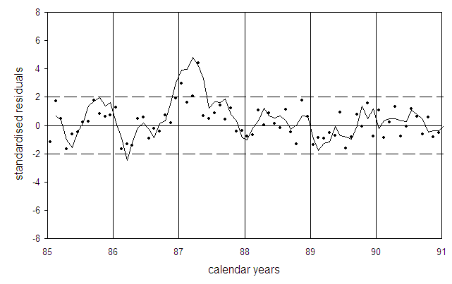
Fig.5: Deviations of observed perinatal mortality rates from the Ukrainian Zhitomir oblast (dots) from the undisturbed long-term trend in units of standard deviations (standardised residuals). The solid line is the three-month moving average, the broken lines show the range of two standard deviations.